Materials+ML Workshop Day 8
![]()
Content for today:
Regression Models Review
- Linear Regression
- High-dimensional Embeddings
- Kernel Machines
Unsupervised Learning
- Feature Selection
- Dimensionality reduction
- Clustering
- Distribution Estimation
- Anomaly Detection
Application: Classifying Superconductors
- Application of unsupervised methods
The Workshop Online Book:
https://cburdine.github.io/materials-ml-workshop/
- A link to our Workshop YouTube playlist is now available
Tentative Week 2 Schedule
| Session | Date | Content |
| Day 6 | 06/16/2025 (2:00-4:00 PM) | Introduction to ML, Supervised Learning |
| Day 7 | 06/17/2025 (2:00-4:00 PM) | Advanced Regression Models |
| Day 8 | 06/18/2025 (2:00-5:00 PM) | Unsupervised Learning, Neural Networks |
| Day 10 | 06/20/2025 (2:00-5:00 PM) | Neural Networks, + Advanced Applications |
Questions
- Regression Models
- Linear Regression
- High-dimensional Embeddings
- Kernel Machines
- Supervised Learning (in general)
Review: Day 7
Multivariate Linear Regression
- Multivariate Linear regression is a type of regression model that estimates a label as a linear combination of features:
We can re-write the linear regression model in vector form:
- Let
($\mathbf{x}$ padded with a 1)
- Let $$\mathbf{w} = \begin{bmatrix} w_0 & w_1 & w_2 & \dots & w_D \end{bmatrix}^T$$
(the weight vector)
- $f(\mathbf{x})$ is just the inner product (i.e. dot product) of these two vectors:
Closed Form Solution:
- Multivariate Linear Regression:
- Above, $\mathbf{X}^+$ denotes the Moore-Penrose inverse (sometimes called the pseudo-inverse) of $\mathbf{X}$.
- If the dataset size $N$ is sufficiently large such that $\mathbf{X}$ has linearly independent columns, the optimal weights can be computed as:
High-Dimensional Embeddings
Often, the trends of $y$ with respect to $\mathbf{x}$ are non-linear, so multivariate linear regression may fail to give good results.
One way of handling this is by embedding the data in a higher-dimensional space using many different non-linear functions:
(The $\phi_j$ are nonlinear functions, and $D_{emb}$ is the embedding dimension)
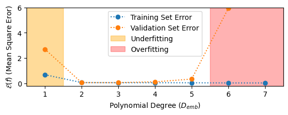
Underfitting and Overfitting
- Finding the best fit of a model requires striking a balance between underfitting and overfitting the data.
- A model underfits the data if it has insufficient degrees of freedom to model the data.
- A model overfits the data if it has too many degrees of freedom such that it fails to generalize well outside of the training data.
Polynomial Regression Example:
Regularization:
- To reduce overfitting, we apply regularization:
Usually, a penalty term is added to the overall model loss function:
$$\text{ Penalty Term } = \lambda \sum_{j} w_j^2 = \lambda(\mathbf{w}^T\mathbf{w})$$
The parameter $\lambda$ is called the regularization parameter
- as $\lambda$ increases, more regularization is applied.
Application: Band Gap Prediction
- Finishing up yesterday's application
Today's Content:
Unsupervised Learning
- Feature Selection
- Dimensionality reduction
- Clustering
- Distribution Estimation
- Anomaly Detection
Unsupervised Learning Models:
Models applied to unlabeled data with the goal of discovering trends, patterns, extracting features, or finding relationships between data.
Deals with datasets of features only
(just $\mathbf{x}$, not $(\mathbf{x},y)$ pairs)
Types of Unsupervised Learning Problems

Feature Selection and Dimensionality Reduction
- Determines which features are the most "meaningful" in explaining how the data is distributed
Sometimes we work with high-dimensional data that is very sparse
Reducing the dimensionality of the data might be necessary
- Reduces computational complexity
- Eliminates unnecessary (or redundant) features
- Can even improve model accuracy
The Importance of Dimensionality
- Dimensionality is an important concept in materials science.
- The dimensionality of a material affects its properties
- Much like materials, the dimensionality of a dataset can say a lot about its properties:
- How complex is the data?
- Are there any "meaningless" or "redundant" features in the dataset?
- Does the data have fewer degrees of freedom than features?
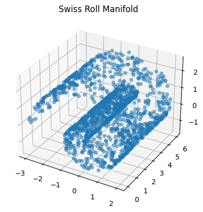
- Sometimes, data can be confined to some low-dimensional manifold embedded in a higher-dimensional space.
Example: The "Swiss Roll" manifold
Review: The Covariance Matrix
- The Covariance Matrix describes the variance of data in more than one dimension:
- $\Sigma_{ii} = \sigma_i^2$: variance in dimension $i$
- $\Sigma_{ij} = \sigma_{ij}$: covariance between dimensions $i$ and $j$
The Correlation Matrix:
- Recall that it is generally a good idea to standardize our data:
- The correlation matrix (denoted $\bar{\Sigma}$) is the covariance matrix of the standardized data:
- The entries of the correlation matrix (in terms of the original data) are:
Interpreting the Correlation Matrix
$$\bar{\Sigma}_{ij} = \frac{1}{N} \sum_{n=1}^N \frac{((\mathbf{x}_n)_i - \mu_i)((\mathbf{x}_n)_j - \mu_j)}{\sigma_i\sigma_j}$$- The diagonal of the correlation matrix consists of $1$s. (Why?)
- The off-diagonal components describe the strength of correlation between feature dimensions $i$ and $j$
- Positive values: positive correlation
- Negative values: negative correlation
- Zero values: no correlation
Principal Components Analysis (PCA)
The eigenvectors of the correlation matrix are called principal components.
The associated eigenvalues describe the proportion of the data variance in the direction of each principal component.
- $D$: Diagonal matrix (eigenvalues along diagonal)
- $P$: Principal component matrix (columns are principal components)
- Since $\bar{\Sigma}$ is symmetric, the principal components $P$ are all orthogonal ($P^{T} = P^{-1}$).
Dimension reduction with PCA
We can project our (normalized) data onto the first $n$ principal components with the largest eigenvalues to reduce the dimensionality of the data, while still keeping most of the variance:
$$\mathbf{z} \mapsto \mathbf{u} = \begin{bmatrix} \mathbf{z}^T\mathbf{p}^{(1)} \\ \mathbf{z}^T\mathbf{p}^{(2)} \\ \vdots \\ \mathbf{z}^T\mathbf{p}^{(n)} \\ \end{bmatrix}$$Exercise: Feature Selection and Dimensionality Reduction
- Applying PCA
Clustering and Distribution Estimation
Clustering methods allow us to identify dense groupings of data.
Distribution Estimation allows us to estimate the probability distribution of the data.
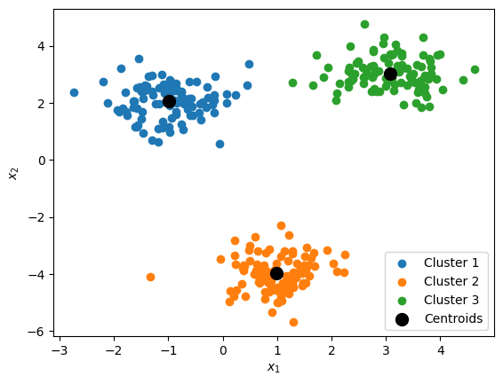
K-Means Clustering:
$k$-means is a popular clustering algorithm that identifies the centerpoints of a specified number of clusters $k$.
These center points are called centroids.
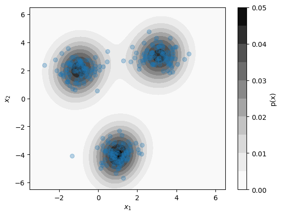
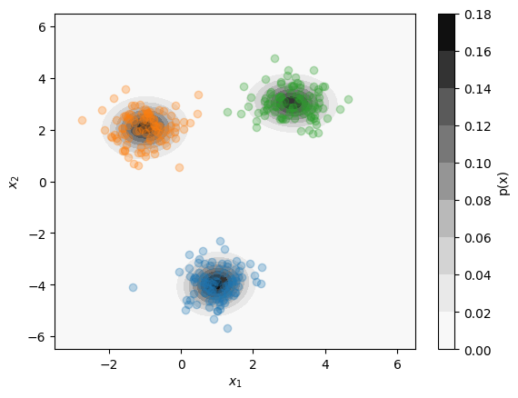
Kernel Density Estimation:
Kernel Density Estimation (KDE) estimates the probability distribution of an entire dataset.
KDE estimates the distribution as a sum of multivariate Gaussian "bumps" at the position of each data point.
Gaussian Mixture Model
A Gaussian Mixture Model (GMM) performs both clustering and distribution estimation simultaneously.
GMM models fit a mixture of multivariate normal distributions to the data.
Exercise: Clustering and Distribution Estimation
- Estimating Density of States with KDE
Application: Classifying Superconductors
- Exploring the distribution of superconducting materials
Recommended Reading:
- Neural Networks
If possible, try to do the exercises. Bring your questions to our next meeting on Friday.
- No meeting tomorrow due to the June 19th Holiday